Forecasting Hotel Revenue: Predicting ADR Fluctuations with ARIMA

Published Jan 13, 2021 by Michael Grogan

Average daily rates (henceforth referred to as ADR) represent the average rate per day paid by a staying customer at a hotel. This is an important metric for a hotel, as it represents the overall profitability of each customer.

In this example, average daily rates for each customer are averaged over a weekly basis and then forecasted using an ARIMA model.

The below analysis is based on data from Antonio, Almeida and Nunes (2019): Hotel booking demand datasets.

Data Manipulation

In this particular dataset, the year and week number for each customer (along with each customer’s recorded ADR value) is provided separately.

Here are the date columns:

Here is the ADR column:

Firstly, the year and week number is combined into one string:

df1 = df['ArrivalDateYear'].map(str) + df['ArrivalDateWeekNumber'].map(str)
print (df1)
df1=pd.DataFrame(df1)

The new column is then concatenated with the ADR column using pandas:

df2 = DataFrame(c, columns= ['ADR']) 
df3=pd.concat([df1, df2], axis = 1)
df3.columns = ['FullDate', 'ADR']

These values are then sorted by date:

df3.sort_values(['FullDate','ADR'], ascending=True)

The next step is to then obtain the average ADR value per week, e.g. for the entry 201527 (which is week 27, year 2015), all the ADR values are averaged, and so on for each subsequent week.

df4 = df3.groupby('FullDate').agg("mean")
df4.sort_values(['FullDate'], ascending=True)

ARIMA

Using this newly formed time series, an ARIMA model can now be used to make forecasts for ADR.

For this model, the first 100 weeks of data are used as training data, while the last 15 weeks are used as test data to be compared with the predictions made by the model.

Here is a plot of the newly formed time series:

From an initial view of the graph, seasonality does seem to be present. However, an autocorrelation function is generated on the training data to verify this.

plot_acf(train_df, lags=60, zero=False);

We can see that the correlations (after seeing a dip roughly between weeks 10 to 45), the autocorrelation peaks once again at lag 52, which implies yearly seasonality. This essentially means that there is a strong correlation between the ADR values recorded every 52 weeks.

Using this information, m=52 is set as the seasonal component in the ARIMA model, and pmdarima is used to automatically select the p, d, q parameters for the model.

>>> Arima_model=pm.auto_arima(train_df, start_p=0, start_q=0, max_p=10, max_q=10, start_P=0, start_Q=0, max_P=10, max_Q=10, m=52, stepwise=True, seasonal=True, information_criterion='aic', trace=True, d=1, D=1, error_action='warn', suppress_warnings=True, random_state = 20, n_fits=30)

Performing stepwise search to minimize aic
 ARIMA(0,1,0)(0,1,0)[52]             : AIC=422.399, Time=0.38 sec
 ARIMA(1,1,0)(1,1,0)[52]             : AIC=inf, Time=5.43 sec
 ARIMA(0,1,1)(0,1,1)[52]             : AIC=inf, Time=6.19 sec
 ARIMA(0,1,0)(1,1,0)[52]             : AIC=inf, Time=4.16 sec
 ARIMA(0,1,0)(0,1,1)[52]             : AIC=inf, Time=2.92 sec
 ARIMA(0,1,0)(1,1,1)[52]             : AIC=inf, Time=6.10 sec
 ARIMA(1,1,0)(0,1,0)[52]             : AIC=414.708, Time=0.22 sec
 ARIMA(1,1,0)(0,1,1)[52]             : AIC=inf, Time=5.70 sec
 ARIMA(1,1,0)(1,1,1)[52]             : AIC=inf, Time=8.11 sec
 ARIMA(2,1,0)(0,1,0)[52]             : AIC=413.878, Time=0.35 sec
 ARIMA(2,1,0)(1,1,0)[52]             : AIC=inf, Time=7.61 sec
 ARIMA(2,1,0)(0,1,1)[52]             : AIC=inf, Time=8.12 sec
 ARIMA(2,1,0)(1,1,1)[52]             : AIC=inf, Time=9.30 sec
 ARIMA(3,1,0)(0,1,0)[52]             : AIC=414.514, Time=0.37 sec
 ARIMA(2,1,1)(0,1,0)[52]             : AIC=415.165, Time=0.78 sec
 ARIMA(1,1,1)(0,1,0)[52]             : AIC=413.365, Time=0.48 sec
 ARIMA(1,1,1)(1,1,0)[52]             : AIC=415.351, Time=24.42 sec
 ARIMA(1,1,1)(0,1,1)[52]             : AIC=inf, Time=16.10 sec
 ARIMA(1,1,1)(1,1,1)[52]             : AIC=inf, Time=26.36 sec
 ARIMA(0,1,1)(0,1,0)[52]             : AIC=411.433, Time=0.36 sec
 ARIMA(0,1,1)(1,1,0)[52]             : AIC=413.418, Time=18.48 sec
 ARIMA(0,1,1)(1,1,1)[52]             : AIC=inf, Time=24.16 sec
 ARIMA(0,1,2)(0,1,0)[52]             : AIC=413.343, Time=0.50 sec
 ARIMA(1,1,2)(0,1,0)[52]             : AIC=415.196, Time=1.16 sec
 ARIMA(0,1,1)(0,1,0)[52] intercept   : AIC=413.377, Time=0.62 sec

Best model:  ARIMA(0,1,1)(0,1,0)[52]          
Total fit time: 178.417 seconds

An ARIMA model configuration of ARIMA(0, 1, 1)(0, 1, 0)[52] is indicated as the model of best fit according to the lowest AIC value.

Now, the model can be used to make predictions for the next 15 weeks, with those predictions compared to the test set:

predictions=pd.DataFrame(Arima_model.predict(n_periods=15), index=test_df)
predictions=np.array(predictions)

Before comparing the predictions with the values from the test set, the predictions are reshaped so as to be in the same format as the test set:

>>> predictions=predictions.reshape(15,-1)
>>> predictions
array([[ 88.0971519 ],
       [103.18056307],
       [117.93678827],
       [121.38546969],
       [112.9812769 ],
       [120.69309927],
       [144.4014371 ],
       [166.36546077],
       [181.69684755],
       [190.12507961],
       [204.36831063],
       [218.85150166],
       [216.59090879],
       [197.74194692],
       [156.98273524]])

Now, the test values can be compared with the predictions on the basis of the root mean squared error (RMSE) — with a lower value indicating less error.

>>> mse = mean_squared_error(test_df, predictions)
>>> rmse = math.sqrt(mse)
>>> print('RMSE: %f' % rmse)
RMSE: 10.093574

>>> np.mean(test_df)
160.492142162915

An RMSE of 10 is obtained compared to a mean of 160. This represents an error of just over 6% of the mean, indicating that the model predicts ADR trends with quite high accuracy.

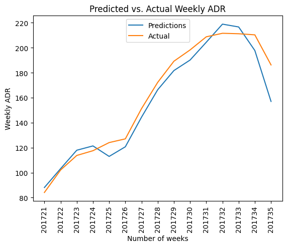
Here is a plot of the predicted vs. actual values.

Based on the RMSE reading and also a visual scan of the data, we can see that the ARIMA model did quite well in predicting ADR trends across the test set.

Conclusion

In this example, we have seen:

How to manipulate time series data using Python
The use of auto_arima to make time series forecasts
How to determine model accuracy using the root mean squared error

The datasets and notebooks for this example are available at the MGCodesandStats GitHub repository, along with further research on this topic.

Data Manipulation

ARIMA

Conclusion

References