ARIMA vs. LSTM: Forecasting Electricity Consumption

Published Dec 12, 2020 by Michael Grogan

In this example, the ARIMA and LSTM models are used to predict electricity consumption patterns for the Dublin City Council Civic Offices, Ireland.

The data in question is sourced from data.gov.ie.

Specifically, the data is provided in terms of kilowatt consumption every 15 minutes.

The analysis takes three stages:

1. Invoke relevant data manipulation procedures in order to aggregate the total kilowatt consumption per day, i.e. form a daily time series.

2. Forecast kilowatt consumption across the test set using an ARIMA model.

3. Generate another forecast across the test set using an LSTM model and examine if the predictions improve.

Data Manipulation

Here is the original set of data loaded into Python.

df = pd.read_csv('dccelectricitycivicsblocks34p20130221-1840.csv', engine='python', skipfooter=3)
df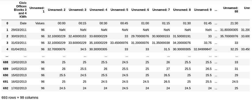

Source: Jupyter Notebook Output

We can see that for each date, the relevant kilowatt consumption is provided across 15-minute intervals.

However, in this instance we wish to forecast the total daily consumption and there is expected to be too much volatility if the time series is formed on a 15-minute basis — so as to make any forecasts quite superficial.

In this regard, the data is sorted on a daily basis:

df2=df.rename(columns=df.iloc[0])
df3=df2.drop(df.index[0])
df3
df3.drop(df3.index[0])
df4=df3.drop('Date', axis=1)
df5=df4.drop('Values', axis=1)
df5
df6=df5.dropna()
df7=df6.values
df7
dataset=np.sum(df7, axis=1, dtype=float)
dataset

The relevant columns are renamed accordingly, and the kilowatt consumption per day is aggregated.

A numpy array containing the aggregated daily data is formed:

array([4981.5001927 , 5166.60016445, 3046.35014537, 3101.10013769,
       4908.60016439, 4858.50017742, 4905.00019836, 4999.95019526,
...
       2383.5       , 4481.5       , 4543.        , 4390.        ,
       4385.        , 4289.5       , 2564.        , 2383.        ])

Here is a plot of the data:

Source: Jupyter Notebook Output

ARIMA

An ARIMA model (or an Autoregressive Integrated Moving Average model) is used to take the components of the time series in question (i.e. p, d, and q parameters), and make new forecasts accordingly.

While pmdarima will be used to select these coordinates automatically, it is important to define the seasonal trend.

The first 80% of the time series (554 observations) are used as training data. Here is a plot of the autocorrelation function as generated on this training set.

Source: Jupyter Notebook Output

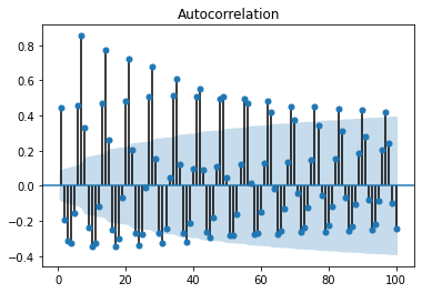
We can see that the highest positive correlation (after the negative correlations) is identified at lag 7. This indicates that there is a strong correlation with the kilowatt reading 7 days after the original.

In this regard, the seasonal component for the ARIMA model is identified as m=7.

Before running the ARIMA model, let’s take a quick look at the 7-day moving average for this time series, in order to better visualise the overall trend.

Source: Jupyter Notebook Output

We can see that the overall kilowatt consumption seems to be decreasing in the first half of the series, while it increases across the second half.

Notably, we can see that there is quite a sharp drop halfway through the series, which clearly marks an anomaly in the series.

This might be due to a power cut or some other event that resulted in a sudden drop in electricity usage. When running the forecasts, we must bear in mind that this “time series shock” would not necessarily be accounted for by the past data.

Using the training data, a stepwise search is now conducted using pmdarima to minimise the AIC value, i.e. select the ARIMA model that shows the lowest AIC.

>>> Arima_model=pm.auto_arima(train_df, start_p=0, start_q=0, max_p=10, max_q=10, start_P=0, start_Q=0, max_P=10, max_Q=10, m=7, stepwise=True, seasonal=True, information_criterion='aic', trace=True, d=1, D=1, error_action='warn', suppress_warnings=True, random_state = 20, n_fits=30)
Performing stepwise search to minimize aic
 ARIMA(0,1,0)(0,1,0)[7]             : AIC=8483.714, Time=0.04 sec
 ARIMA(1,1,0)(1,1,0)[7]             : AIC=8421.989, Time=0.12 sec
 ARIMA(0,1,1)(0,1,1)[7]             : AIC=8319.248, Time=0.34 sec
 ARIMA(0,1,1)(0,1,0)[7]             : AIC=8360.091, Time=0.10 sec
 ARIMA(0,1,1)(1,1,1)[7]             : AIC=inf, Time=0.78 sec
 ARIMA(0,1,1)(0,1,2)[7]             : AIC=inf, Time=1.36 sec
 ARIMA(0,1,1)(1,1,0)[7]             : AIC=8328.690, Time=0.27 sec
 ARIMA(0,1,1)(1,1,2)[7]             : AIC=inf, Time=2.29 sec
 ARIMA(0,1,0)(0,1,1)[7]             : AIC=8451.400, Time=0.18 sec
 ARIMA(1,1,1)(0,1,1)[7]             : AIC=inf, Time=0.81 sec
 ARIMA(0,1,2)(0,1,1)[7]             : AIC=inf, Time=0.75 sec
 ARIMA(1,1,0)(0,1,1)[7]             : AIC=8415.537, Time=0.09 sec
 ARIMA(1,1,2)(0,1,1)[7]             : AIC=inf, Time=1.16 sec
 ARIMA(0,1,1)(0,1,1)[7] intercept   : AIC=8321.247, Time=1.30 sec

Best model:  ARIMA(0,1,1)(0,1,1)[7]          
Total fit time: 9.588 seconds

The most suitable ARIMA model is identified as ARIMA(0,1,1)(0,1,1)[7].

Now, a prediction can be made for the next 126 days, with the predictions compared to the actual results obtained across the test set.

prediction=pd.DataFrame(Arima_model.predict(n_periods=126), index=test_df)
prediction=np.array(prediction)

The predictions are reshaped in order to ensure the same format across the test set and the predictions:

prediction=prediction.reshape(126,-1)

The root mean squared error is calculated:

>>> mse = mean_squared_error(test_df, prediction)
>>> rmse = math.sqrt(mse)
>>> print('RMSE: %f' % rmse)
RMSE: 1288.000396

The mean kilowatt consumption across the test set came in at 3,862. Given that the RMSE error accounts for 33% of the size of the mean, this indicates that the ARIMA model could be doing a better job at forecasting electricity consumption.

To get a more intuitive look at what is going on, let’s plot the predictions and test data.

Source: Jupyter Notebook Output

We can see that the ARIMA model has picked up the seasonal trend of the series quite well. That said, the peak consumption predictions in the first half of the graph appear to be quite a bit higher than the actual.

Moreover, we see that the model fails to capture the drop in kilowatt consumption between roughly days 70–80 across the test set. This anomaly may be contributing to the sizeable error we are seeing for the RMSE value, as RMSE is designed to penalise errors on outliers more heavily.

Note that manually configuring the ARIMA model, i.e. implementing manual selection of the p, d, q coordinates showed an improvement in the forecast accuracy, with an RMSE of 965. Here are some more detailed results in a follow-up article.

LSTM

An LSTM model is now implemented on this set of data to examine if the forecast accuracy improves when using this approach.

The data was manipulated in the same way as above initially, i.e. a daily time series was formed by aggregating the kilowatt consumption every 15 minutes in the space of one day.

The data is split into training and test data:

train_size = int(len(df) * 0.8)
test_size = len(df) - train_size
train, test = df[0:train_size,:], df[train_size:len(df),:]

A dataset matrix is formed:

def create_dataset(df, previous=1):
    dataX, dataY = [], []
    for i in range(len(df)-previous-1):
        a = df[i:(i+previous), 0]
        dataX.append(a)
        dataY.append(df[i + previous, 0])
    return np.array(dataX), np.array(dataY)

Data Normalization

The data is normalized in order to allow the LSTM model to interpret the data properly.

However, there is a big caveat when it comes to implementing this procedure. The training and test sets must be split separately (as above) before conducting the scaling procedure on each set separately.

A common mistake when implementing an LSTM model is to simply scale the whole dataset. This is erroneous as the scaler will use the values from the test set as a baseline for the scale, resulting in data leakage back to the training set.

For instance, let us suppose that a hypothetical training set has a scale from 1–1000, and the hypothetical test set has a scale from 1–1200. MaxMinScaler will reduce the scale to a number between 0–1. Should the data be scaled across both the training and test set concurrently, then MaxMinScaler will use the 1–1200 scale as the baseline for the training set as well. This means that the new scale across the training set has been compromised by the test set, resulting in unreliable forecasts.

Thus, the data in our example is scaled as follows:

scaler = MinMaxScaler(feature_range=(0, 1))
train = scaler.fit_transform(train)
train
test = scaler.fit_transform(test)
test

LSTM Model Configuration

Now that the data is scaled, a lookback period needs to be implemented, i.e. how many prior periods we wish for the LSTM model to take into account when forecasting at time t.

After trial and error, a lookback period of 5 showed the lowest RMSE when forecasting.

lookback = 5
X_train, Y_train = create_dataset(train, lookback)
X_test, Y_test = create_dataset(test, lookback)

The input is then reshaped to be of the format samples, time steps, features.

The LSTM network is defined and trained:

# Generate LSTM network
model = tf.keras.Sequential()
model.add(LSTM(4, input_shape=(1, lookback)))
model.add(Dense(1))
model.compile(loss='mean_squared_error', optimizer='adam')
history=model.fit(X_train, Y_train, validation_split=0.2, epochs=100, batch_size=1, verbose=2)

Here is a plot of the training and validation loss:

Source: Jupyter Notebook Output

The predictions are generated and then converted back to the original scale (after having been previously converted using MinMaxScaler):

trainpred = model.predict(X_train)
testpred = model.predict(X_test)
trainpred = scaler.inverse_transform(trainpred)
Y_train = scaler.inverse_transform([Y_train])
testpred = scaler.inverse_transform(testpred)
Y_test = scaler.inverse_transform([Y_test])
predictions = testpred

Now, the prediction accuracy can be computed by comparing the predictions to the actual test data.

Firstly, here is a plot of the predicted vs actual data.

Source: Jupyter Notebook Output

The RMSE value is calculated.

>>> mse = mean_squared_error(Y_test, predictions)
>>> rmse = sqrt(mse)
>>> print('RMSE: %f' % rmse)
RMSE: 410.116102

The mean value across the test set is 3,909. The size of the RMSE accounts for 10% of the mean, which means the model shows superior performance to ARIMA in predicting electricity consumption trends.

From the graph, it is also notable that the LSTM model was adept at forecasting the period where there was a lower consumption level than normal. This would be somewhat expected given that the LSTM is a one-step prediction model, i.e. kilowatt consumption at time t cannot be predicted without having the values for the previous five weeks — it is not a long-range forecast.

That said, the LSTM model has been more effective at accounting for the volatility in the series.

Conclusion

In this example, we have seen:

• How to conduct data manipulation using pandas

• Configuring an ARIMA model to make long-term forecasts

• One-step ahead forecasting with the LSTM model

• How to gauge prediction accuracy using RMSE

Many thanks for your time, and the relevant GitHub repository with the dataset and code examples can be found here.

References

• data.gov.ie: Energy Consumption (Gas and Electricity) Civic Offices 2009–2012

• Machine Learning Mastery: Time Series Forecasting Performance Measures With Python